- Published on
VLOOKUP like the Pros
- Authors

- Name
- David Krevitt
- Link
- Data App Enthusiast
- Get in Touch
Welcome to Cacheworthy
This post is a vestige of this blog's previous life as CIFL (2015 - 2023), which covered building analytics pipelines for internal reporting. When migrating to Cacheworthy and a focus on data applications, we found this post too helpful to remove - hope you enjoy it!
Curious about data applications? Meet Cacheworthy.VLOOKUP is the gateway drug of Google Sheets formulas.
A little taste of it you'll be hooked on the power of spreadsheets - it's a small, simple formula that will save you hours when manipulating or analyzing data.
This post will help teach you how to write a number of VLOOKUP formula variants: make a copy of the accompanying cheat sheet to follow along.
Let's dive into the VLOOKUPS!
- Step by step VLOOKUP tutorial
- 1. The basic VLOOKUP formula
- 2. Using VLOOKUP on a range (ARRAYFORMULA)
- 3. VLOOKUP from another Sheet
- 4. VLOOKUP on multiple criteria with ARRAYFORMULA
- 5. Reverse VLOOKUP
- 6. HLOOKUP
- Your turn!
Step by step VLOOKUP tutorial
If you prefer a video walkthrough, follow along here throughout the post:
1. The basic VLOOKUP formula
In its simplest form, VLOOKUP allows you to find a value from a table, based on the value in another column:
- A Twitter handle based on the user's name
- A company name based on their website URL
If you have a big table with raw data, VLOOKUP is your first weapon to start plucking out specific values.
For example, a large dataset of Tweets that you want to extract data from.
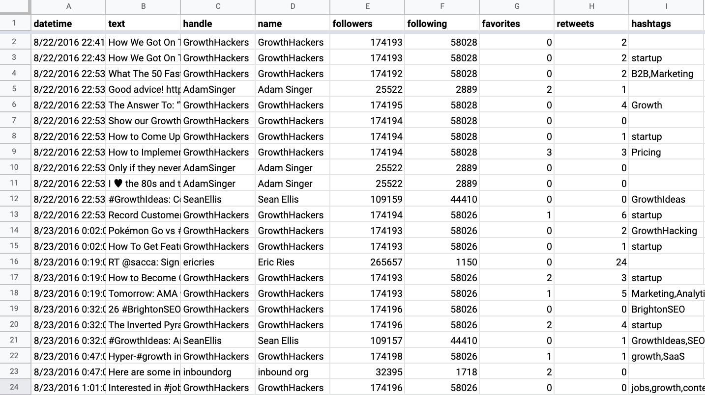
How it works The order of the formula is tricky if you've never used it - but be patient, and allow yourself to not understand it the first time:
=VLOOKUP(value to lookup, data range, column number to pull, 0)
Let's start with a question (based on data in the 'Sample Tweets' dataset tab):
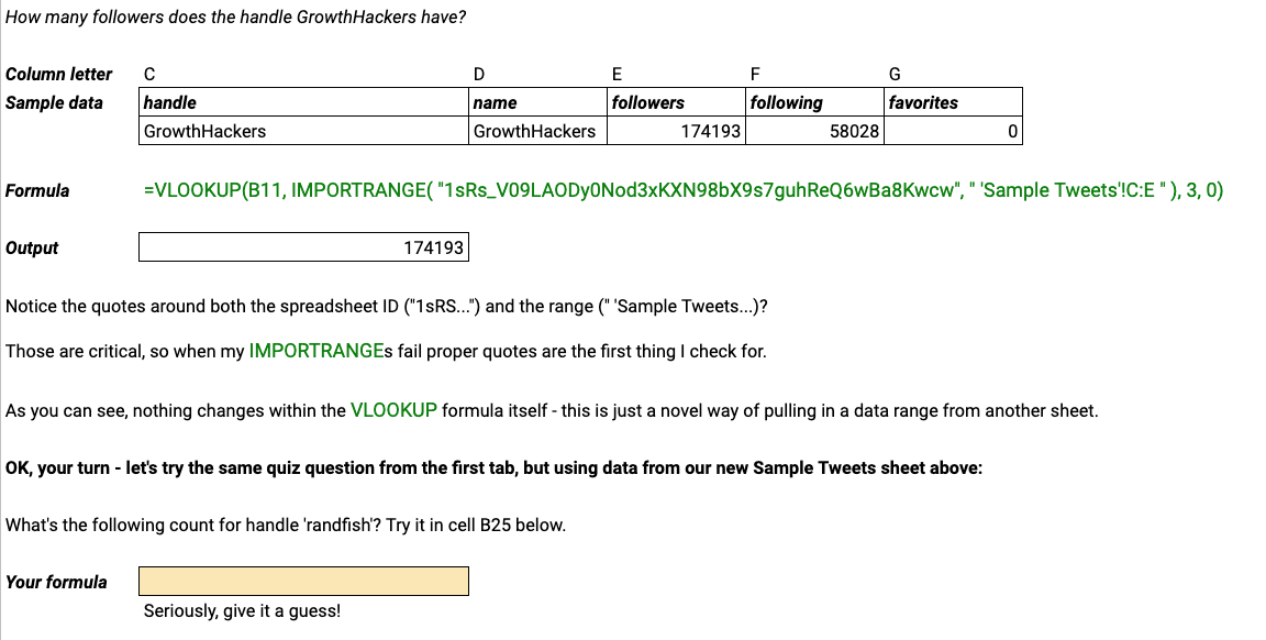
How many followers does the handle GrowthHackers have?
The VLOOKUP we'd need to answer that is:
=VLOOKUP(B10, ‘Sample Tweets’!C:E, 3, 0)
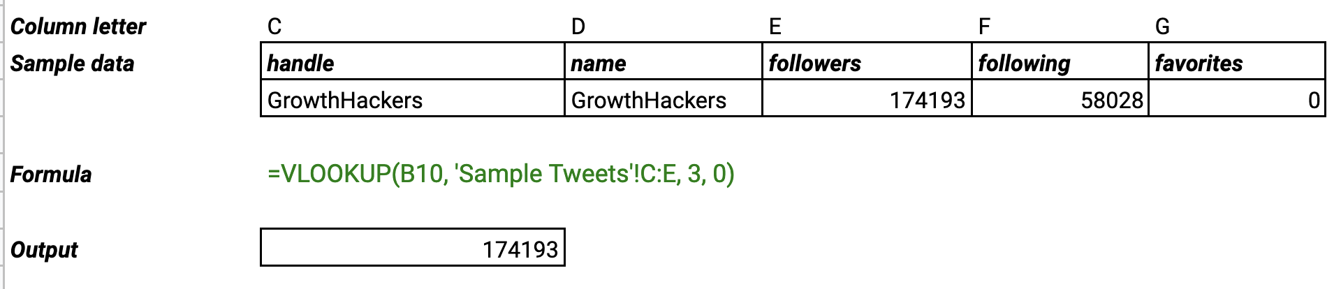
Super important: The value that you're looking up (GrowthHackers, or cell B10 in this case) MUST BE in the first column of your data range.
Our data lives in rows C:E of the 'Sample Tweets' tab, so that's our second parameter. And we want to pull the 3rd column over.
It's also important to note that VLOOKUP returns the first value it finds - so if you have multiple rows containing your search term, it will only pull the first one.
2. Using VLOOKUP on a range (ARRAYFORMULA)
It's pretty rare that you'll use a VLOOKUP in isolation.
Usually, once you write one, you'll want to apply it to an entire range of cells.
For example, you'll have a bunch of Twitter handles in one column, and you'll want to pull follower counts for all of them.
Let's try doing that, by combining it with ARRAYFORMULA. Think about ARRAYFORMULA as a replacement for copy-paste within spreadsheets.
How it works
There’s one key to understanding ARRAYFORMULA: everything must be a range.
You can’t just run a VLOOKUP on cell A2 - you’ve got to pass the entire array (A2:A, or a subset like A2:A6).
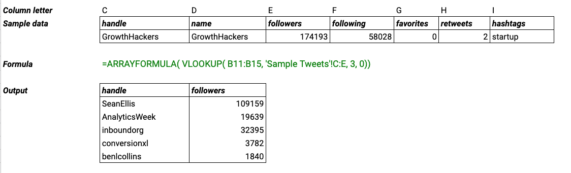
=ARRAYFORMULA( VLOOKUP( A2:A, data!$A:$C, 3, 0))
That’s really all there is to it. You write a formula as you normally would (VLOOKUP in this case), rewrite any individual cells (A2) as ranges (A2:A), and wrap the entire thing in ARRAYFORMULA().
Let's try the question from above - pulling follower counts for a column of handles:
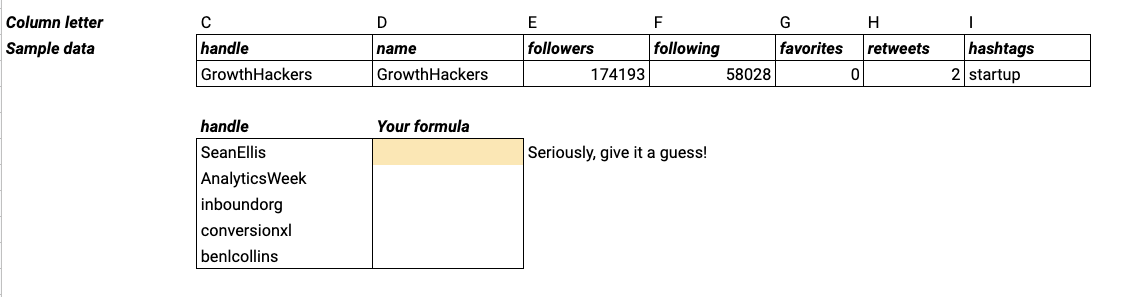
Let's try a tougher question, to test your newfound VLOOKUP + ARRAYFORMULA skills:
What hashtags (from column I) appeared in the first Tweets from the same list of handles above?
Write once, run everywhere. ARRAYFORMULA allows you to set a lookup across an entire column, without copying and pasting the formula into each cell - keeping your Sheets nice and clean.
3. VLOOKUP from another Sheet
One of my favorite things about Google Sheets, is that you can easily pass data across different sheets.
For example, if you have a sheet that collects form responses, you probably don't want to be mucking it up with some analysis.
But you definitely do want to analyze that form data. The IMPORTRANGE function lets you do that, guilt-free, in another sheet.
How it works
As formulas go, it's a simple one:
=IMPORTRANGE( "spreadsheet ID from URL" , "range" )
The spreadsheet ID can be pulled from the source sheet's URL, between /d/ and /edit:
docs.google.com/spreadsheets/d/ 1-nX4WJuHrTMRlDZKmWClG-Pv8sVT3QlHEd7J8xFmhlI /edit
And the range is the same as if you were pulling data from within the same sheet. For example, 'Getting Started'!A:B to pull the first two columns of the first tab in this sheet.
Diving in
Let's run back the same question, except this time answer it using data in this sheet (which contains the same data from the 'Sample Tweets' tab here):
=VLOOKUP(B11, IMPORTRANGE( ‘1sRs\_V09LAODy0Nod3xKXN98bX9s7guhReQ6wBa8Kwcw’, ‘ ‘Sample Tweets’!C:E ‘ ), 3, 0)
This is where Google Sheets separates itself from Excel.
Since any Google Sheet can import data (using IMPORTRANGE) from any other Sheet, you can run it on data from outside your current Sheet.
4. VLOOKUP on multiple criteria with ARRAYFORMULA
Often you'll wish VLOOKUP was less rigid - like when you want to match values from *two* columns instead of just one.
Instead of modifying the VLOOKUP formula itself, situations like these require getting creative.
If you want to match two columns in a lookup, you'll have to combine those two values into one - and also combine them within the range that you're looking up against.
To do this, we'll use a couple helpers: the &, and ARRAYFORMULA.
Let's try pulling the first tweet by GrowthHackers that uses the hashtag 'startups':
=VLOOKUP( B11 & C11, { ARRAYFORMULA (‘Sample Tweets’!C:C & ‘Sample Tweets’!I:I ), ‘Sample Tweets’!B:B }, 2, 0)
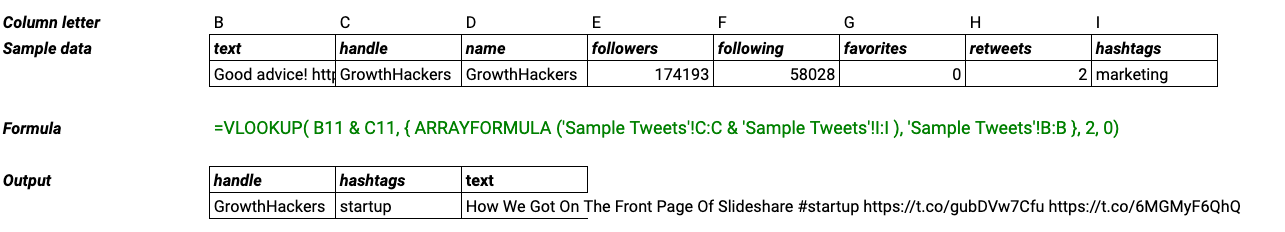
In the first parameter (B11 & C11), we combine the handle & hashtag to become one value: GrowthHackersstartup.
Then, in the lookup range, we combine columns C and I from 'Sample Tweets', which contain the handle and hashtag, to form the first column.
{ ARRAYFORMULA ('Sample Tweets'!C:C & 'Sample Tweets'!I:I ), 'Sample Tweets'!B:B }
Layering in the tweet text (column B) creates a two-column lookup range - so that we can pull the tweet text matching both the GrowtHackers handle and the startup hashtag.
Because VLOOKUP is so simple, it’s very easy to trick into doing thing it’s not specifically built for. You can combine multiple columns (concatenate them essentially) before running the lookup, which will trick the formula to look for matches on both criteria.
5. Reverse VLOOKUP
In the last tab, we learned to get creative with the order and combination of our VLOOKUP columns by combining and ARRAYFORMULA.
That trick comes in handy if you're looking to pull columns that are behind your lookup column - some would call this a reverse VLOOKUP.
This lets you get around one of the formula's peskiest combinations, and be more creative with your formula writing.
Let's give it a shot, and lookup the date of AdamSinger's first tweet:
=VLOOKUP ( B11, {‘Sample Tweets’!C:C, ‘Sample Tweets’!A:A }, 2, 0)
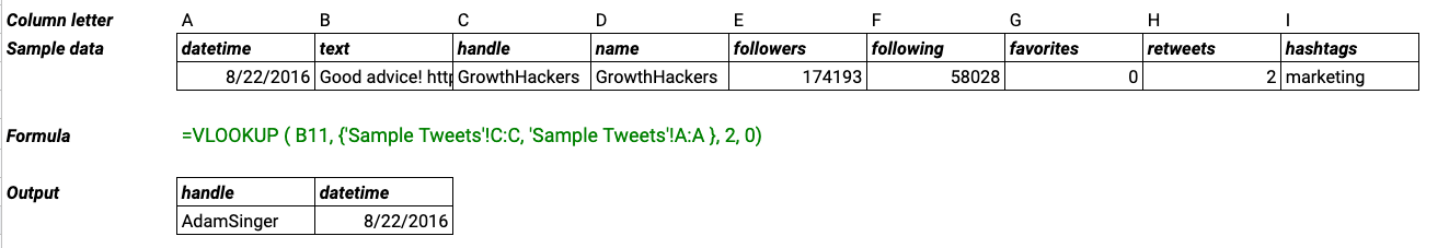
See how you combine the range in reverse order? Just by embedding the two columns within curly braces , separated by a comma.
That allows you to perform a VLOOKUP on the range as usual - the rest of the formula is vanilla.
One of the pains with VLOOKUP is that it can only look up values left-to-right - the value you’re looking up against has to be in the leftmost column of your range.
But - what if you rearrange your, er, range? Using the handy curly braces { } in Google Sheets, you can recombine columns in an order that works with VLOOKUP.
6. HLOOKUP
What if your data lives in rows instead of columns?
This often happens when you're looking at historical data at work - where month names might live in the headers, and accounts in each row:
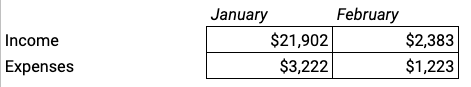
In this situation, VLOOKUP wouldn't be the best formula for looking up, say, the expenses in February.
Because you'd have to know exactly which column February was in, and historical columns have a habit of moving around on you without warning.
Instead, let's turn to VLOOKUPs cousin, HLOOKUP, which will let us lookup based on the column name, and pull a given row.
What it we wanted to pull the second tweet from the handle column below?
=HLOOKUP( ‘handle’, B11:G13, 3, 0)
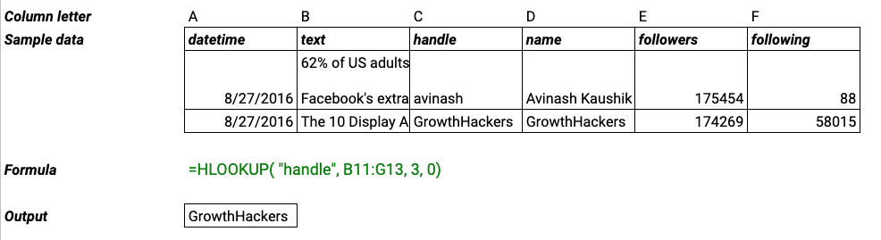
The syntax is more or less the same as VLOOKUP - you reference:
- a value to lookup
- the lookup range
- the row number to pull
Notice that, just like VLOOKUP, the index for row numbers to lookup starts at 1 - so if you want to pull the 2nd tweet in this case, it's actually 3rd in the index (because of the header row).
If your data is oriented the wrong way for VLOOKUP, you can instead use it’s close cousin, HLOOKUP.
For example, if you have dates in the header row of your Sheet, and you’re looking to pull the value in a specific row, for a specific date, you’d HLOOKUP for that date, and then pull the Nth row.
[su_divider top="no" style="dashed" divider_color="#dddddd" size="2" margin="50"]
Your turn!
It's tough to get the most out of this post without using the cheat sheet, so make sure you grab your copy here.
If you liked this post, please make sure to check us out on YouTube where we post tutorial videos like this one.