9 Google Sheets Formulas to Master

There’s endless combinations of Google Sheets formulas you could use to automate your work.

Trying to master them all would be a complete waste of your time.

Why?

To master Google Sheets formulas, you only really need a handful.

9, to be exact.

I’m going to walk you through each of the 9 key Google Sheets formulas that you need to become a master.

• MAKE A COPY OF THE WORKBOOK

I’m not asking for your email address (I know that’s annoying). But if you do get value from this post, I’m hoping you will check out my YouTube Channel where I have even better tutorials.

• Subscribe to my YouTube Channel

Let’s get into the need-to-know formulas!

1. ARRAYFORMULA

This one confused me for a long time. But once I figured out how to use ARRAYFORMULA, I’ll never go back.

This is a true instrument of laziness.

It allows you to write a formula once, and apply it to an entire row or column.

No more copy and pasting across a sheet – and when that one arrayformula breaks, you only have one cell to check (instead of 1000 if you’re copy-pasting).

How it works

There’s one key to understanding ARRAYFORMULA: everything must be a range. You can’t just run a vlookup on cell A2 – you’ve got to pass the entire array (A2:A, or some section like A2:A6).

=ARRAYFORMULA( VLOOKUP( A2:A, data!$A:$C, 3, 0))

That’s really all there is to ARRAYFORMULA. You write a formula as you normally would (VLOOKUP in this case), rewrite any individual cells (A2) as ranges (A2:A), and wrap the entire thing in ARRAYFORMULA().

When to use it

Anytime you want to run the same formula across multiple cells. Think about arrayformula as a replacement for copy-paste within spreadsheets.

I find myself using it most often when I want to populate an entire column.

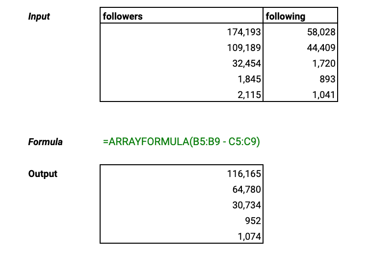
For example, using our sample Twitter data, what if we wanted to subtract the number of followers from number following, for the entire column?

Input

Formula

=ARRAYFORMULA(B5:B9 - C5:C9)

Output 

2. SPLIT

SPLIT helps you separate a string of text, separated by a character (like a comma), into separate cells.

The delimiter (separating character) can be any value – a space, a comma, a pipe (“|”), a phrase (“www”).

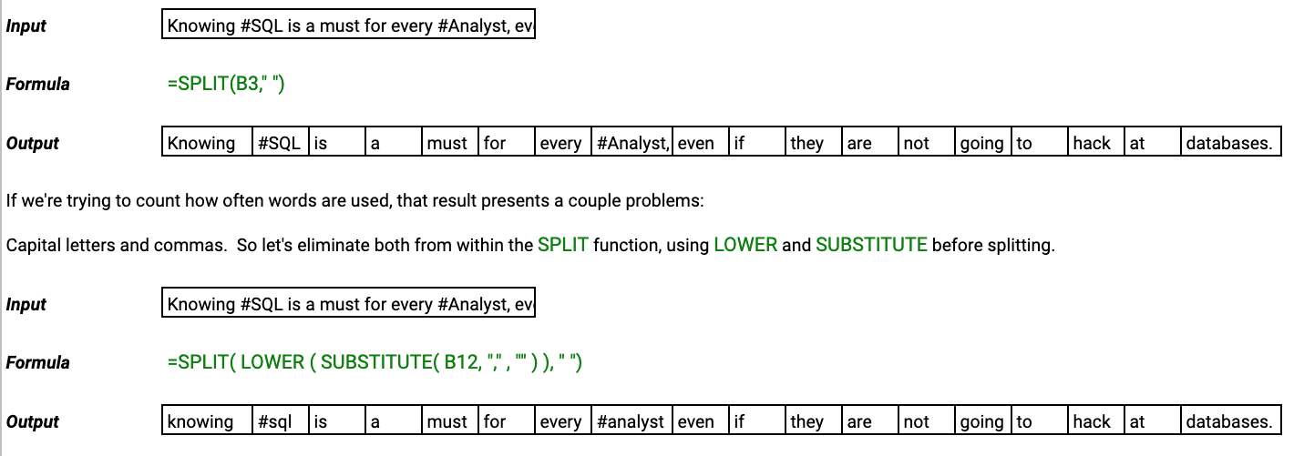
For example, let’s try splitting a Tweet out into words:

Input

Knowing #SQL is a must for every #Analyst, even if they are not going to hack at databases.

Formula

=SPLIT(B3," ")

Output

3. INDEX

If you ever want to pull a specific value from a range of cells – INDEX is your sniper.

You pass it a range, a row, and a column, and it returns the value present there.

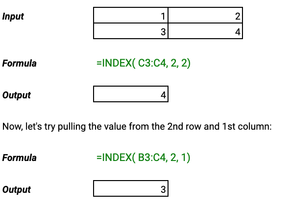
To demonstrate, let’s take the 2 x 2 range below. What if we wanted to pull the value in the 2nd row and 2nd column?

Input

Formula

=INDEX( B3:C4, 2, 2)

Output

4

Now, let’s try pulling the value from the 2nd row and 1st column:

Formula

=INDEX( B3:C4, 2, 1)

Output

3

4. LEFT and RIGHT

LEFT and RIGHT allow you to slice off a segment of text from either side of a cell.

Each of them only takes two arguments:

LEFT(text, # of characters) or RIGHT(text, # of characters).

Let’s take a date string, for example:

Mon Aug 22 22:58:54 +0000 2016

Using LEFT or RIGHT, you could pull out any of the individual date values: the day, the month, the date, the hour or the year.

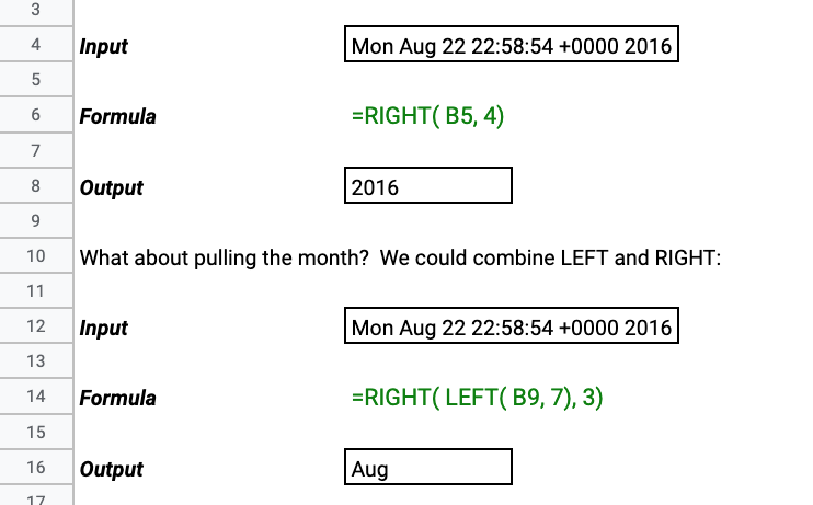
Let’s start with pulling just the year:

Input

Mon Aug 22 22:58:54 +0000 2016

Formula

=RIGHT( B5, 4)

Output

2016

What about pulling the month? We could combine LEFT and RIGHT:

Input

Mon Aug 22 22:58:54 +0000 2016

Formula

=RIGHT( LEFT( B9, 7), 3)

Output

Aug

5. IF and IFERROR

If you’ve used spreadsheets before, you’ve likely written an IF function.

They let you embed logic into your formulas – and keep formulas in your sheet from running when they don’t need to:

=IF(A2="", do nothing, run this function)

This simple IF statement keeps the function from running if A2 is blank – if there’s nothing for the formula to process, no reason to run it!

This keeps your sheets clean and fast – running a bunch of formulas unnecessarily will slow things down.

Input

Blank cell

Formula

=IF( B5="", "Don't run the function", "Run the function")

Output

Don’t run the function

IF has a cousin, IFERROR, that further helps bulletproof our sheets.

There are many functions, like VLOOKUP or QUERY, that will throw error messages when they fail:

Error – Did not find value in VLOOKUP evaluation.

These make your sheets ugly, and may cause other calculations downstream to fail – so I use IFERROR to set the output in the event of an error.

Input

Formula

=IFERROR( VLOOKUP( "lisa", B11:C12, 2, 0), "No result")

Output

No result

Both IF and IFERROR become really powerful when used with ARRAYFORMULA, since they allow you to keep entire columns or rows clean with one formula.

6. Working with Dates

Making dates update automatically in your spreadsheets is *the biggest* consistent timesaver I’ve found.

There’s one key function that is the keystone for all date automation: TODAY.

TODAY returns, er, today’s date, which lets you easily build date ranges. Say we wanted to pull the last 7 days for a report:

Formula

=TODAY() - 7

=TODAY()

Output (as of publishing)

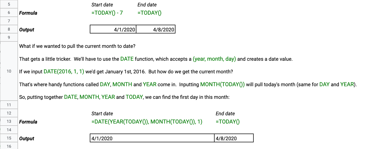
What if we wanted to pull the current month to date?

That gets a little tricker. We’ll have to use the DATE function, which accepts a (year, month, day) and creates a date value.

If we input DATE(2016, 1, 1) we’d get January 1st, 2016. But how do we get the current month?

That’s where handy functions called DAY, MONTH and YEAR come in. Inputting MONTH(TODAY()) will pull today’s month (same for DAY and YEAR).

So, putting together DATE, MONTH, YEAR and TODAY, we can find the first day in this month:

Formula

=DATE(YEAR(TODAY()), MONTH(TODAY()), 1)

=TODAY()

Output (as of publishing)

What would you guess the WEEKDAY function does? That’s right – it pulls the weekday that a date falls on.

But instead of telling you Saturday or Sunday, it returns a number (1 = Sunday).

Say you wanted to pull sales numbers for only Sundays, WEEKDAY is your best friend.

7. TEXT

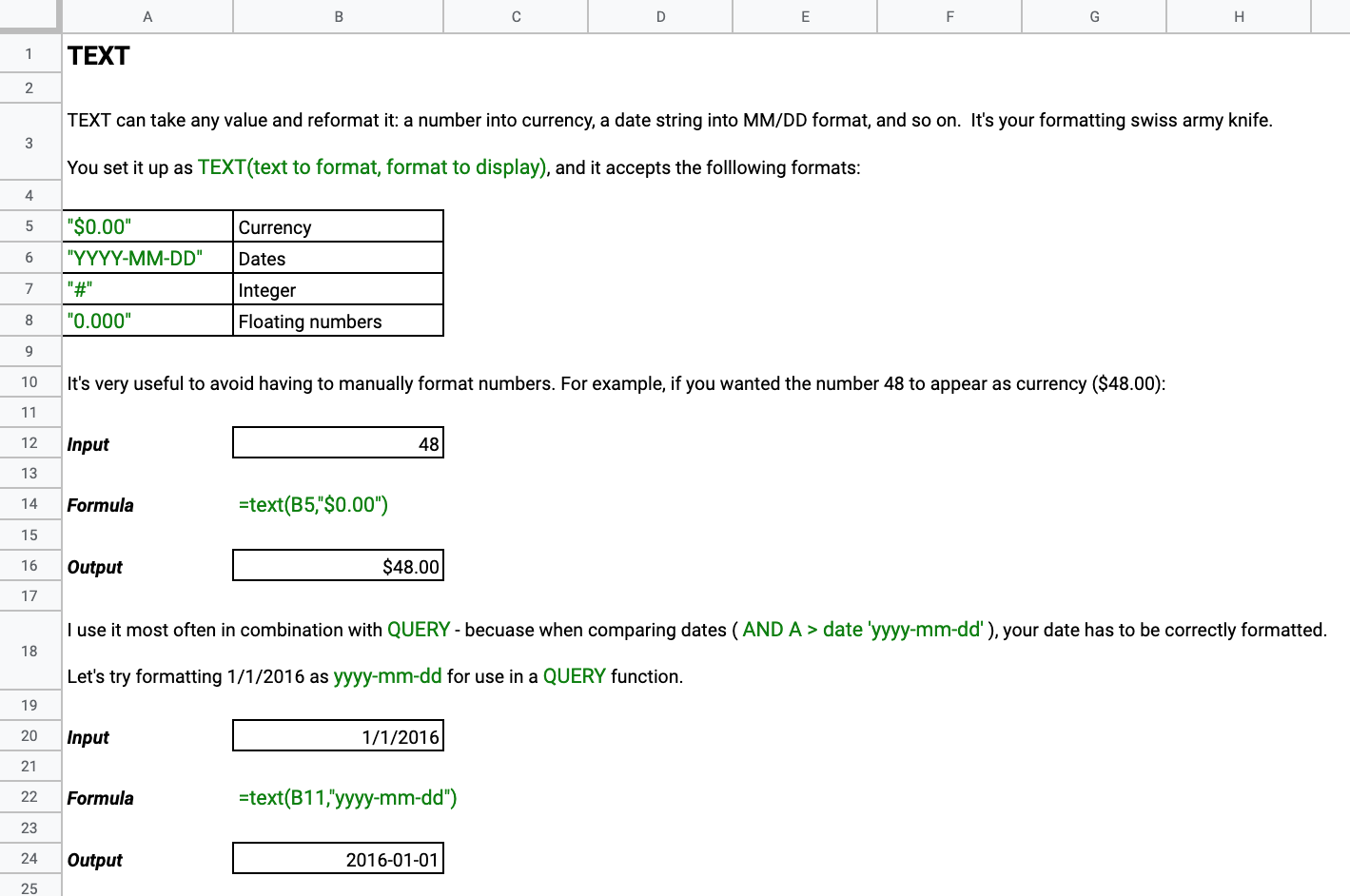
TEXT can take any value and reformat it: a number into currency, a date string into MM/DD format, and so on. It’s your formatting swiss army knife.

You set it up as TEXT(text to format, format to display), and it accepts the folllowing formats:

"$0.00"

"YYYY-MM-DD"

"#"

"0.000"

It’s very useful to avoid having to manually format numbers. For example, if you wanted the number 48 to appear as currency ($48.00):

Input

48

Formula

=TEXT ( B5 , "$0.00" )

Output

$48.00

I use it most often in combination with QUERY – becuase when comparing dates ( AND A > date ‘yyyy-mm-dd’ ), your date has to be correctly formatted.

Let’s try formatting 1/1/2017 as yyyy-mm-dd for use in a QUERY function.

Input

1/1/2017

Formula

=TEXT ( B11 , "yyyy-mm-dd" )

Output

2017-01-01

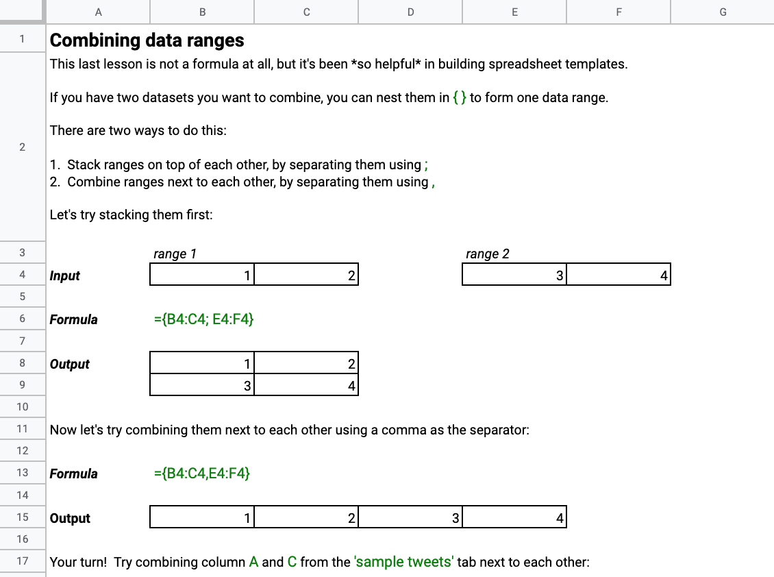
8. Combining Data Ranges

This is not a formula at all, but it’s been *so helpful* in building spreadsheet templates.

If you have two datasets you want to combine, you can nest them in { } to form one data range.

There are two ways to do this:

1. Stack ranges on top of each other, by separating them using ;
2. Combine ranges next to each other, by separating them using ,

Let’s try stacking them first:

Input

Formula

={B4:C4 ; E4:F4}

Output

Now let’s try combining them next to each other using a comma as the separator:

Formula

={B4:C4 , E4:F4}

Output

9. QUERY

The big kahuna of Sheets functions.  QUERY lets you combine all of them into one powerful ball of Google Sheets formula magic.

Say we’re looking at Twitter data, and we want to answer the question:

Who tweeted the word ‘dashboard’?

Our next question will probably be:

Who tweeted ‘dashboard’ the most this week? Last week?

Using QUERY lets us explore all of those questions from roughly the same formula, without having to string formulas together (like you’d have to do with FILTER, REGEXMATCH and others).

https://codingisforlosers.com/google-sheets-query-function/

** If you’ve ever used SQL, then you’ll recognize Google queries. **

That’s all!

I know that’s a lot of material to pick up off the bat, so feel free to grab the cheat sheet and learn at your leisure.

• MAKE A COPY OF THE CHEAT SHEET WORKBOOK

If you’re ready to dive wayyy deeper, also check out all of the Coding is for Losers courses on mastering Google Sheets.